7.13. Implementing Knight’s Tour

The search algorithm we will use to solve the knight’s tour problem is called depth first search (DFS). Whereas the breadth first search algorithm discussed in the previous section builds a search tree one level at a time, a depth first search creates a search tree by exploring one branch of the tree as deeply as possible. In this section we will look at two algorithms that implement a depth first search. The first algorithm we will look at directly solves the knight’s tour problem by explicitly forbidding a node to be visited more than once. The second implementation is more general, but allows nodes to be visited more than once as the tree is constructed. The second version is used in subsequent sections to develop additional graph algorithms.

The depth first exploration of the graph is exactly what we need in order to find a path that has exactly 63 edges. We will see that when the depth first search algorithm finds a dead end (a place in the graph where there are no more moves possible) it backs up the tree to the next deepest vertex that allows it to make a legal move.

The knightTour function takes four parameters: n, the current depth in the search tree; path, a list of vertices visited up to this point; u, the vertex in the graph we wish to explore; and limit the number of nodes in the path. The knightTour function is recursive. When the knightTour function is called, it first checks the base case condition. If we have a path that contains 64 vertices, we return from knightTourwith a status of True, indicating that we have found a successful tour. If the path is not long enough we continue to explore one level deeper by choosing a new vertex to explore and calling knightTourrecursively for that vertex.

DFS also uses colors to keep track of which vertices in the graph have been visited. Unvisited vertices are colored white, and visited vertices are colored gray. If all neighbors of a particular vertex have been explored and we have not yet reached our goal length of 64 vertices, we have reached a dead end. When we reach a dead end we must backtrack. Backtracking happens when we return from knightTour with a status of False. In the breadth first search we used a queue to keep track of which vertex to visit next. Since depth first search is recursive, we are implicitly using a stack to help us with our backtracking. When we return from a call to knightTour with a status of False, in line 11, we remain inside the while loop and look at the next vertex in nbrList.

Listing 3

from pythonds.graphs import Graph, Vertex
def knightTour(n,path,u,limit):
        u.setColor('gray')
        path.append(u)
        if n < limit:
            nbrList = list(u.getConnections())
            i = 0
            done = False
            while i < len(nbrList) and not done:
                if nbrList[i].getColor() == 'white':
                    done = knightTour(n+1, path, nbrList[i], limit)
                i = i + 1
            if not done:  # prepare to backtrack
                path.pop()
                u.setColor('white')
        else:
            done = True
        return done

Let’s look at a simple example of knightTour in action. You can refer to the figures below to follow the steps of the search. For this example we will assume that the call to the getConnections method on line 6 orders the nodes in alphabetical order. We begin by calling knightTour(0,path,A,6)

knightTour starts with node A Figure 3. The nodes adjacent to A are B and D. Since B is before D alphabetically, DFS selects B to expand next as shown in Figure 4. Exploring B happens when knightTouris called recursively. B is adjacent to C and D, so knightTour elects to explore C next. However, as you can see in Figure 5 node C is a dead end with no adjacent white nodes. At this point we change the color of node C back to white. The call to knightTour returns a value of False. The return from the recursive call effectively backtracks the search to vertex B (see Figure 6). The next vertex on the list to explore is vertex D, so knightTour makes a recursive call moving to node D (see Figure 7). From vertex D on, knightTourcan continue to make recursive calls until we get to node C again (see Figure 8, Figure 9, and Figure 10). However, this time when we get to node C the test n < limit fails so we know that we have exhausted all the nodes in the graph. At this point we can return True to indicate that we have made a successful tour of the graph. When we return the list, path has the values [A,B,D,E,F,C], which is the the order we need to traverse the graph to visit each node exactly once.

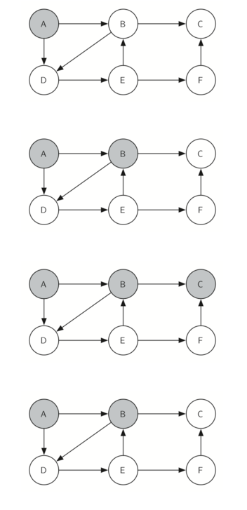
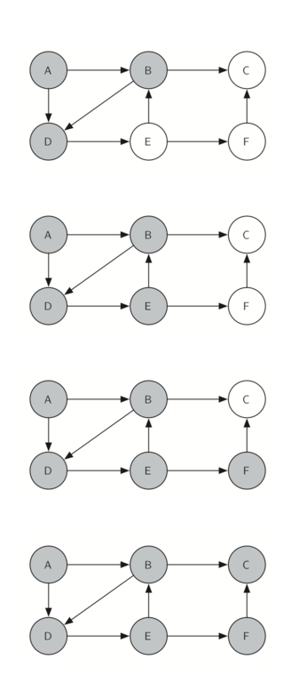
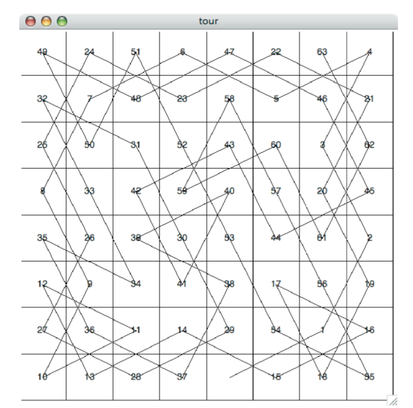
Figure 11 shows you what a complete tour around an eight-by-eight board looks like. There are many possible tours; some are symmetric. With some modification you can make circular tours that start and end at the same square.

7.14. Knight’s Tour Analysis

There is one last interesting topic regarding the knight’s tour problem, then we will move on to the general version of the depth first search. The topic is performance. In particular, knightTour is very sensitive to the method you use to select the next vertex to visit. For example, on a five-by-five board you can produce a path in about 1.5 seconds on a reasonably fast computer. But what happens if you try an eight-by-eight board? In this case, depending on the speed of your computer, you may have to wait up to a half hour to get the results! The reason for this is that the knight’s tour problem as we have implemented it so far is an exponential algorithm of size $O (k N) "> O (k N)$ , where N is the number of squares on the chess board, and k is a small constant. Figure 12 can help us visualize why this is so. The root of the tree represents the starting point of the search. From there the algorithm generates and checks each of the possible moves the knight can make. As we have noted before the number of moves possible depends on the position of the knight on the board. In the corners there are only two legal moves, on the squares adjacent to the corners there are three and in the middle of the board there are eight. Figure 13 shows the number of moves possible for each position on a board. At the next level of the tree there are once again between 2 and 8 possible next moves from the position we are currently exploring. The number of possible positions to examine corresponds to the number of nodes in the search tree.

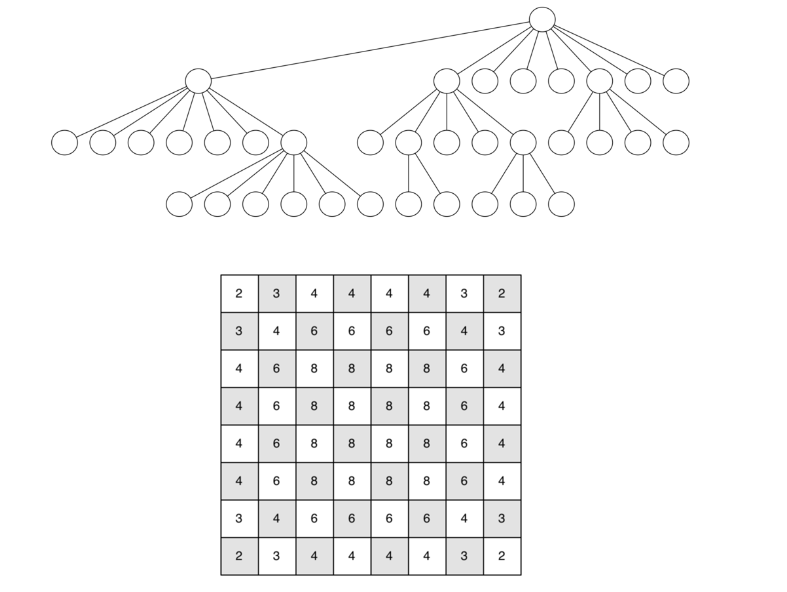
We have already seen that the number of nodes in a binary tree of height N is $2 N + 1 - 1 "> 2 N + 1 - 1$ . For a tree with nodes that may have up to eight children instead of two the number of nodes is much larger. Because the branching factor of each node is variable, we could estimate the number of nodes using an average branching factor. The important thing to note is that this algorithm is exponential: $k N + 1 - 1 "> k N + 1 - 1$ , where $k "> k$ is the average branching factor for the board. Let’s look at how rapidly this grows! For a board that is 5x5 the tree will be 25 levels deep, or N = 24 counting the first level as level 0. The average branching factor is $k = 3.8 "> k = 3.8$ So the number of nodes in the search tree is $3.8 25 - 1 "> 3.8 25 - 1$ or $3.12 \times 1014 "> 3.12 \times 1014$ . For a 6x6 board, $k = 4.4 "> k = 4.4$ , there are $1.5 \times 1023 "> 1.5 \times 1023$ nodes, and for a regular 8x8 chess board, $k = 5.25 "> k = 5.25$ , there are $1.3 \times 1046 "> 1.3 \times 1046$ . Of course, since there are multiple solutions to the problem we won’t have to explore every single node, but the fractional part of the nodes we do have to explore is just a constant multiplier which does not change the exponential nature of the problem. We will leave it as an exercise for you to see if you can express $k "> k$ as a function of the board size.

Luckily there is a way to speed up the eight-by-eight case so that it runs in under one second. In the listing below we show the code that speeds up the knightTour. This function (see Listing 4), called orderbyAvail will be used in place of the call to u.getConnections in the code previously shown above. The critical line in the orderByAvail function is line 10. This line ensures that we select the vertex to go next that has the fewest available moves. You might think this is really counter productive; why not select the node that has the most available moves? You can try that approach easily by running the program yourself and inserting the line resList.reverse() right after the sort.

The problem with using the vertex with the most available moves as your next vertex on the path is that it tends to have the knight visit the middle squares early on in the tour. When this happens it is easy for the knight to get stranded on one side of the board where it cannot reach unvisited squares on the other side of the board. On the other hand, visiting the squares with the fewest available moves first pushes the knight to visit the squares around the edges of the board first. This ensures that the knight will visit the hard-to-reach corners early and can use the middle squares to hop across the board only when necessary. Utilizing this kind of knowledge to speed up an algorithm is called a heuristic. Humans use heuristics every day to help make decisions, heuristic searches are often used in the field of artificial intelligence. This particular heuristic is called Warnsdorff’s algorithm, named after H. C. Warnsdorff who published his idea in 1823.

Listing 4

def orderByAvail(n):
    resList = []
    for v in n.getConnections():
        if v.getColor() == 'white':
            c = 0
            for w in v.getConnections():
                if w.getColor() == 'white':
                    c = c + 1
            resList.append((c,v))
    resList.sort(key=lambda x: x[0])
    return [y[1] for y in resList]

7.15. General Depth First Search

The knight’s tour is a special case of a depth first search where the goal is to create the deepest depth first tree, without any branches. The more general depth first search is actually easier. Its goal is to search as deeply as possible, connecting as many nodes in the graph as possible and branching where necessary.

It is even possible that a depth first search will create more than one tree. When the depth first search algorithm creates a group of trees we call this a depth first forest. As with the breadth first search our depth first search makes use of predecessor links to construct the tree. In addition, the depth first search will make use of two additional instance variables in the Vertex class. The new instance variables are the discovery and finish times. The discovery time tracks the number of steps in the algorithm before a vertex is first encountered. The finish time is the number of steps in the algorithm before a vertex is colored black. As we will see after looking at the algorithm, the discovery and finish times of the nodes provide some interesting properties we can use in later algorithms.

The code for our depth first search is shown in Listing 5. Since the two functions dfs and its helper dfsvisit use a variable to keep track of the time across calls to dfsvisit we chose to implement the code as methods of a class that inherits from the Graph class. This implementation extends the graph class by adding a time instance variable and the two methods dfs and dfsvisit. Looking at line 11 you will notice that the dfs method iterates over all of the vertices in the graph calling dfsvisit on the nodes that are white. The reason we iterate over all the nodes, rather than simply searching from a chosen starting node, is to make sure that all nodes in the graph are considered and that no vertices are left out of the depth first forest. It may look unusual to see the statement for aVertex in self, but remember that in this case self is an instance of the DFSGraph class, and iterating over all the vertices in an instance of a graph is a natural thing to do.

Listing 5

from pythonds.graphs import Graph
class DFSGraph(Graph):
    def __init__(self):
        super().__init__()
        self.time = 0

    def dfs(self):
        for aVertex in self:
            aVertex.setColor('white')
            aVertex.setPred(-1)
        for aVertex in self:
            if aVertex.getColor() == 'white':
                self.dfsvisit(aVertex)

    def dfsvisit(self,startVertex):
        startVertex.setColor('gray')
        self.time += 1
        startVertex.setDiscovery(self.time)
        for nextVertex in startVertex.getConnections():
            if nextVertex.getColor() == 'white':
                nextVertex.setPred(startVertex)
                self.dfsvisit(nextVertex)
        startVertex.setColor('black')
        self.time += 1
        startVertex.setFinish(self.time)

Although our implementation of bfs was only interested in considering nodes for which there was a path leading back to the start, it is possible to create a breadth first forest that represents the shortest path between all pairs of nodes in the graph. We leave this as an exercise. In our next two algorithms we will see why keeping track of the depth first forest is important.

The dfsvisit method starts with a single vertex called startVertex and explores all of the neighboring white vertices as deeply as possible. If you look carefully at the code for dfsvisit and compare it to breadth first search, what you should notice is that the dfsvisit algorithm is almost identical to bfsexcept that on the last line of the inner for loop, dfsvisit calls itself recursively to continue the search at a deeper level, whereas bfs adds the node to a queue for later exploration. It is interesting to note that where bfs uses a queue, dfsvisit uses a stack. You don’t see a stack in the code, but it is implicit in the recursive call to dfsvisit.

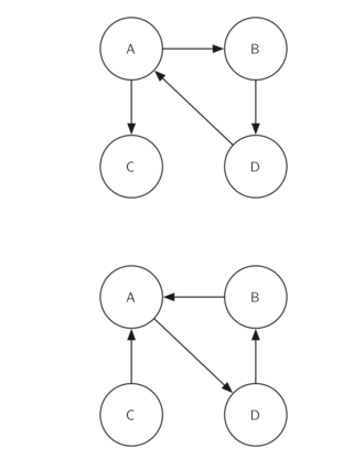
The following sequence of figures illustrates the depth first search algorithm in action for a small graph. In these figures, the dotted lines indicate edges that are checked, but the node at the other end of the edge has already been added to the depth first tree. In the code this test is done by checking that the color of the other node is non-white.

The search begins at vertex A of the graph (Figure 14). Since all of the vertices are white at the beginning of the search the algorithm visits vertex A. The first step in visiting a vertex is to set the color to gray, which indicates that the vertex is being explored and the discovery time is set to 1. Since vertex A has two adjacent vertices (B, D) each of those need to be visited as well. We’ll make the arbitrary decision that we will visit the adjacent vertices in alphabetical order.

Vertex B is visited next (Figure 15), so its color is set to gray and its discovery time is set to 2. Vertex B is also adjacent to two other nodes (C, D) so we will follow the alphabetical order and visit node C next.

Visiting vertex C (Figure 16) brings us to the end of one branch of the tree. After coloring the node gray and setting its discovery time to 3, the algorithm also determines that there are no adjacent vertices to C. This means that we are done exploring node C and so we can color the vertex black, and set the finish time to 4. You can see the state of our search at this point in Figure 17.

Since vertex C was the end of one branch we now return to vertex B and continue exploring the nodes adjacent to B. The only additional vertex to explore from B is D, so we can now visit D (Figure 18) and continue our search from vertex D. Vertex D quickly leads us to vertex E (Figure 19). Vertex E has two adjacent vertices, B and F. Normally we would explore these adjacent vertices alphabetically, but since B is already colored gray the algorithm recognizes that it should not visit B since doing so would put the algorithm in a loop! So exploration continues with the next vertex in the list, namely F (Figure 20).

Vertex F has only one adjacent vertex, C, but since C is colored black there is nothing else to explore, and the algorithm has reached the end of another branch. From here on, you will see in Figure 21 throughFigure 25 that the algorithm works its way back to the first node, setting finish times and coloring vertices black.

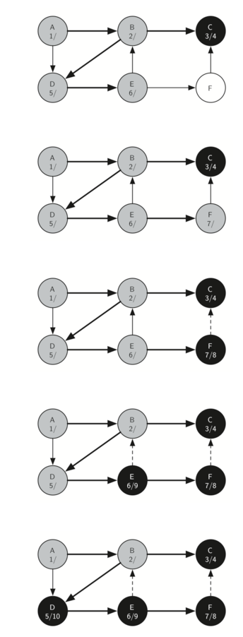
The starting and finishing times for each node display a property called the parenthesis property. This property means that all the children of a particular node in the depth first tree have a later discovery time and an earlier finish time than their parent. Figure 26 shows the tree constructed by the depth first search algorithm.

7.16. Depth First Search Analysis

The general running time for depth first search is as follows. The loops in dfs both run in $O (V) "> O (V)$ , not counting what happens in dfsvisit, since they are executed once for each vertex in the graph. In dfsvisit the loop is executed once for each edge in the adjacency list of the current vertex. Since dfsvisit is only called recursively if the vertex is white, the loop will execute a maximum of once for every edge in the graph or $O (E) "> O (E)$ . So, the total time for depth first search is $O (V + E) "> O (V + E)$ .

7.17. Topological Sorting

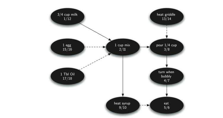
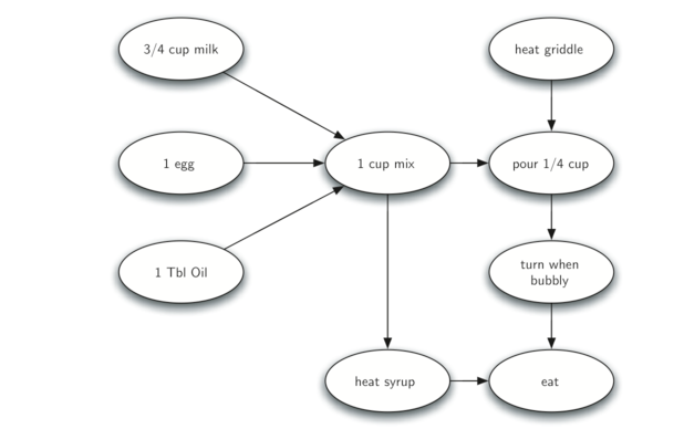
To demonstrate that computer scientists can turn just about anything into a graph problem, let’s consider the difficult problem of stirring up a batch of pancakes. The recipe is really quite simple: 1 egg, 1 cup of pancake mix, 1 tablespoon oil, and $34 "> 3 4$ cup of milk. To make pancakes you must heat the griddle, mix all the ingredients together and spoon the mix onto a hot griddle. When the pancakes start to bubble you turn them over and let them cook until they are golden brown on the bottom. Before you eat your pancakes you are going to want to heat up some syrup. Figure 27 illustrates this process as a graph.

The difficult thing about making pancakes is knowing what to do first. As you can see from Figure 27 you might start by heating the griddle or by adding any of the ingredients to the pancake mix. To help us decide the precise order in which we should do each of the steps required to make our pancakes we turn to a graph algorithm called the topological sort.

A topological sort takes a directed acyclic graph and produces a linear ordering of all its vertices such that if the graph $G "> G$ contains an edge $(v, w) "> (v, w)$ then the vertex $v "> v$ comes before the vertex $w "> w$ in the ordering. Directed acyclic graphs are used in many applications to indicate the precedence of events. Making pancakes is just one example; other examples include software project schedules, precedence charts for optimizing database queries, and multiplying matrices.

The topological sort is a simple but useful adaptation of a depth first search. The algorithm for the topological sort is as follows:

Call dfs(g) for some graph g. The main reason we want to call depth first search is to compute the finish times for each of the vertices.
Store the vertices in a list in decreasing order of finish time.
Return the ordered list as the result of the topological sort.

Figure 28 shows the depth first forest constructed by dfs on the pancake-making graph shown in Figure

Finally, Figure 29 shows the results of applying the topological sort algorithm to our graph. Now all the ambiguity has been removed and we know exactly the order in which to perform the pancake making steps.

7.18. Strongly Connected Components

For the remainder of this chapter we will turn our attention to some extremely large graphs. The graphs we will use to study some additional algorithms are the graphs produced by the connections between hosts on the Internet and the links between web pages. We will begin with web pages.

Search engines like Google and Bing exploit the fact that the pages on the web form a very large directed graph. To transform the World Wide Web into a graph, we will treat a page as a vertex, and the hyperlinks on the page as edges connecting one vertex to another. Figure 30 shows a very small part of the graph produced by following the links from one page to the next, beginning at Luther College’s Computer Science home page. Of course, this graph could be huge, so we have limited it to web sites that are no more than 10 links away from the CS home page.

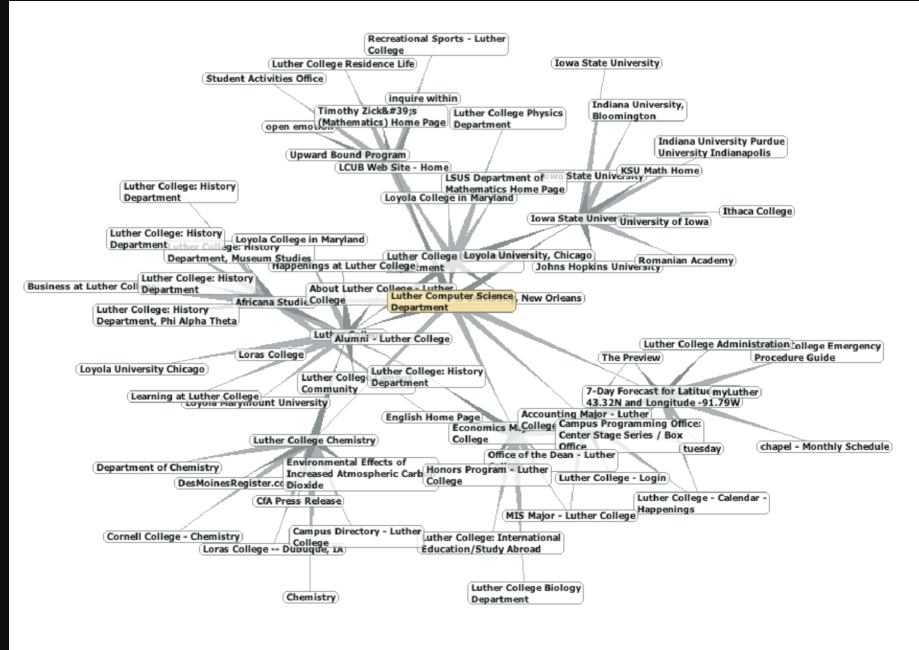
If you study the graph in Figure 30 you might make some interesting observations. First you might notice that many of the other web sites on the graph are other Luther College web sites. Second, you might notice that there are several links to other colleges in Iowa. Third, you might notice that there are several links to other liberal arts colleges. You might conclude from this that there is some underlying structure to the web that clusters together web sites that are similar on some level.

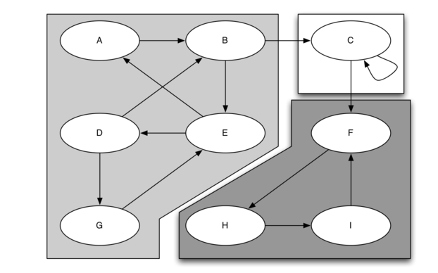
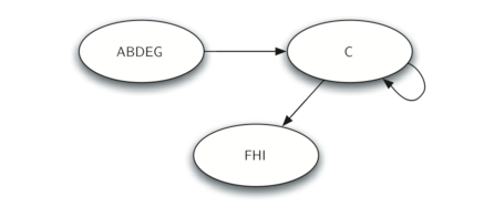
One graph algorithm that can help find clusters of highly interconnected vertices in a graph is called the strongly connected components algorithm (SCC). We formally define a strongly connected component, $C "> C$ , of a graph $G "> G$ , as the largest subset of vertices $C \subset V "> C \subset V$ such that for every pair of vertices $v, w \in C "> v, w \in C$ we have a path from $v "> v$ to $w "> w$ and a path from $w "> w$ to $v "> v$ . Figure 27 shows a simple graph with three strongly connected components. The strongly connected components are identified by the different shaded areas.

Once the strongly connected components have been identified we can show a simplified view of the graph by combining all the vertices in one strongly connected component into a single larger vertex. The simplified version of the graph in Figure 31 is shown in Figure 32.

Once again we will see that we can create a very powerful and efficient algorithm by making use of a depth first search. Before we tackle the main SCC algorithm we must look at one other definition. The transposition of a graph $G "> G$ is defined as the graph $G T "> G T$ where all the edges in the graph have been reversed. That is, if there is a directed edge from node A to node B in the original graph then $G T "> G T$ will contain and edge from node B to node A. Figure 33 and Figure 34 show a simple graph and its transposition.

Look at the figures again. Notice that the graph in Figure 33 has two strongly connected components. Now look at Figure 34. Notice that it has the same two strongly connected components.

We can now describe the algorithm to compute the strongly connected components for a graph.

Call dfs for the graph $G "> G$ to compute the finish times for each vertex.
Compute $G T "> G T$ .
Call dfs for the graph $G T "> G T$ but in the main loop of DFS explore each vertex in decreasing order of finish time.
Each tree in the forest computed in step 3 is a strongly connected component. Output the vertex ids for each vertex in each tree in the forest to identify the component.

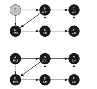
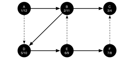
Let’s trace the operation of the steps described above on the example graph in Figure 31. Figure 35 shows the starting and finishing times computed for the original graph by the DFS algorithm. Figure 36 shows the starting and finishing times computed by running DFS on the transposed graph.

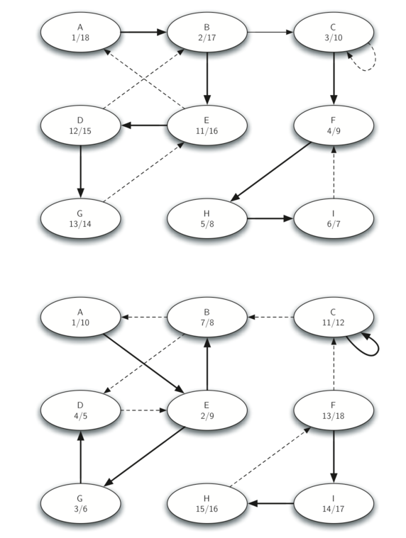
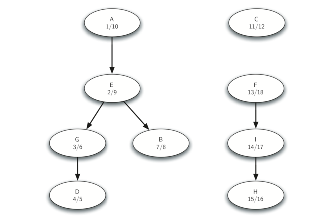
Finally, Figure 37 shows the forest of three trees produced in step 3 of the strongly connected component algorithm. You will notice that we do not provide you with the Python code for the SCC algorithm, we leave writing this program as an exercise.

Graphs and Graph Algorithms - Part 2

7.13. Implementing Knight’s Tour The search algorithm we will use to solve the knight’s